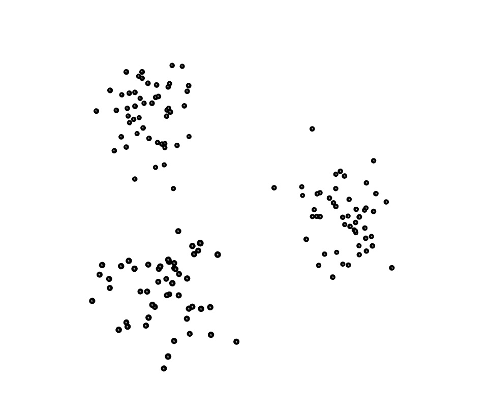
k-Means Algorithms
Given a dataset of n-rows select k-rows such that k≤n.
These are the seed rows for creating k clusters within the dataset. The efficacy of the method is determined by how well chosen these initial cells are. Should they be too close together, say two rows within a cluster that is relatively distant from another cluster, then it is likely that the cluster will be partitioned into two, even if that is less than optimal. Should there be k clusters within the dataset, then such an event will result in one of the two of the other ‘real’ clusters being assigned to a single partition.
The efficaciousness of the clustering is also limited to selecting the correct number of clusters natural to the dataset. Should there be an undercount, then multiple clusters may be grouped together based on the initial rows that were selected. Should there be an overcount, then one or more natural clusters will be partitioned into multiple sectors.
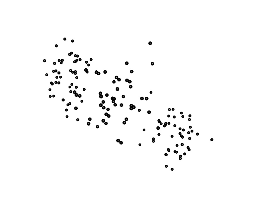 Viewed from the wrong perspective it may not be clear as to how elements within the data set are related to each other, and may even seem to be correlated to the degree that they form a single class | |
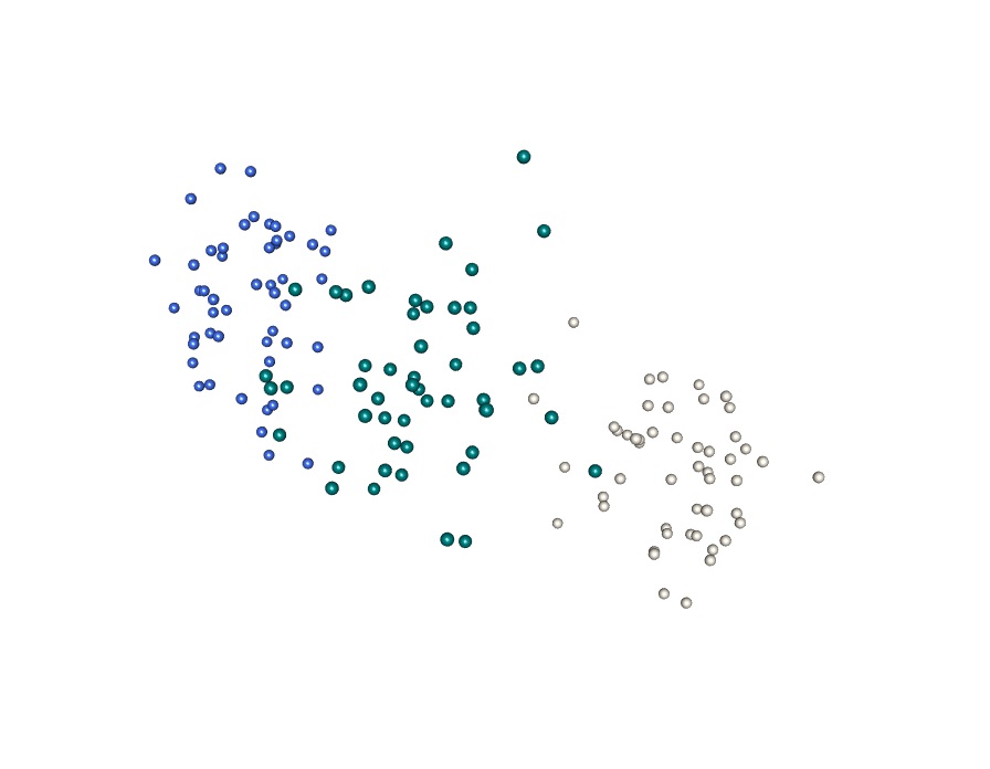 Even where differences are readily observable in the data they may be obscured by applying the wrong framework to the data set being analysed | 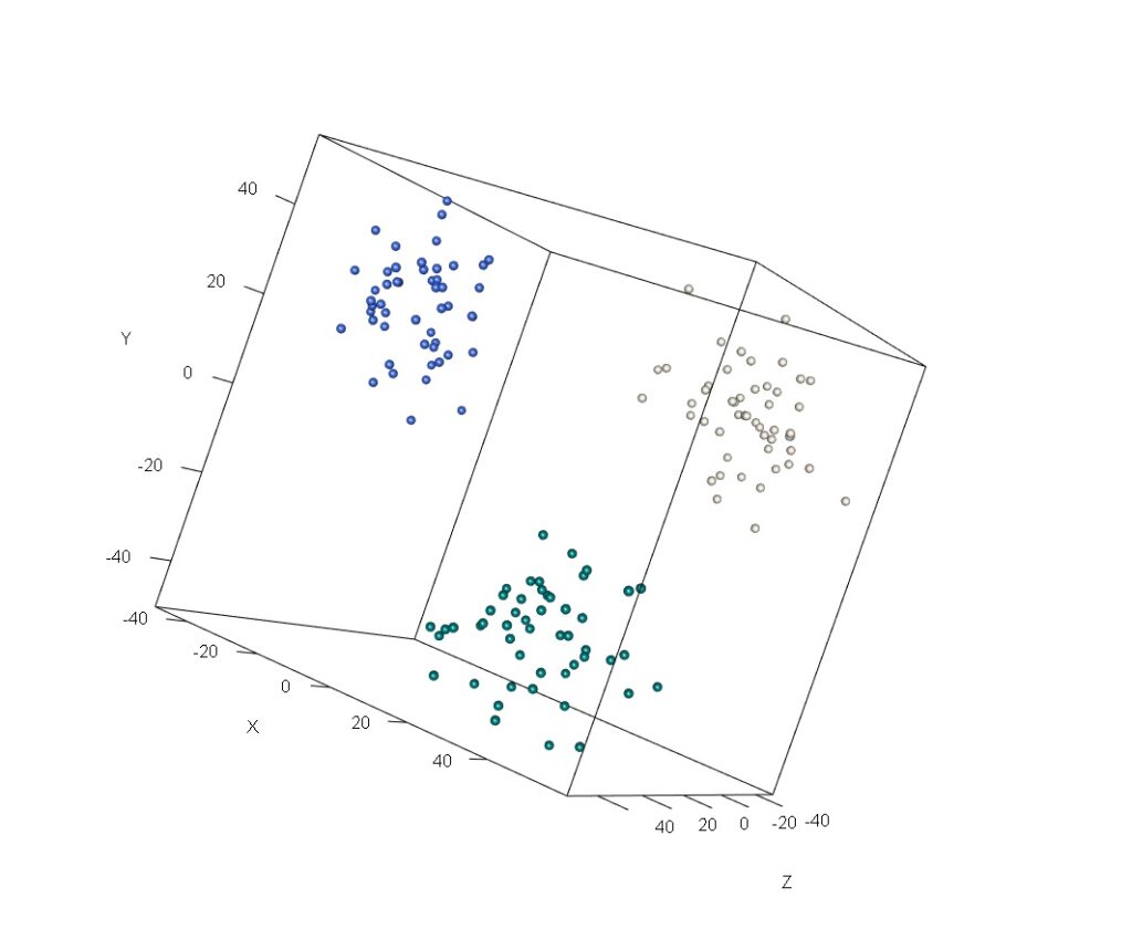 Using the appropriate transformations can be beneficial when seeking to identify relevant commonalities and differences between data objects Using the appropriate transformations can be beneficial when seeking to identify relevant commonalities and differences between data objects |
While the initial rows may be picked at random, there are better means to select rows which consider the distance from the previously selected rows, and the sparseness of the data within. There is little that can be done procedurally regarding the selecting of the wrong k/number of clusters to find. k-Means is both complete clustering and non-overlapping, as a result no cluster will be empty, and every row will be assigned to one, and only one, cluster.
Once the initial rows have been chosen, the next closest row to each joins the initial row in it’s subset of the total dataset. The average/center of each partition is calculated. The row that is not assigned to the dataset which is closest to the centre of each cluster joins that cluster. If no unassigned rows are close to a cluster then the cluster stabilises. A new center is calculated for each cluster. The process iterates until all rows have been assigned, or some other threshold is reached – consider a pair, or more, of clusters that may swap an equidistant point between them indefinitely.
In creating a condition that can be used to identify an optimal point to break the process, sum of squares is often used.

∀ i ϵ k, find the sum of the squared deviations of all points within i, from the average/ideal point that is the center of partition i. Square it to remove the negative signs. Then sum across all clusters. A good fit will minimise this calculation. It may be useful to run k-Means multiple times and then select the ‘best fit’ example.
k-Means is non-deterministic, is is possible/likely that different iterations will assign particular rows to different clusters based on the initial conditions.
k-Means is most useful when:
Clusters are distinct (well separated), and within clusters they are dense, compact clouds.
It is good when working with high-dimensional data as this increases the distances between rows quickly.
k-Means is also computationally efficient
However….
Data types matter: The calculation of a mean is a limitation when it comes to categorical data.
k value is parameterised: If the k is inappropriate, the algorithm will not be useful for correcting the error, at best the errors will be minimised given the constraint that there must be k clusters.
Outliers matter: As k-means uses the mean of the cluster as the reference point, it is vulnerable to outliers shifting the mean from the true centre of the cluster. Using this mean as a proxy for the data objects within the cluster will lead to the referent object being biased rather than the true centre.
Data structure matters. Partitioning clusters which have concave distributions may be difficult where there clusters are poorly segregated.
Distribution matters: Where there is an overlap between clusters (caused by a high degree of variance around a particular cluster center, relative to the inter-group distance) then the cluster which members of the overlapping area between clusters can be unstable.
Variations of k-Means
k-Medoid tracks the median row within the cluster, making the algorithm less sensitive to the influence of outliers. This acts to limit the deviation of the cluster mean from the true centre
K++ means: The first cluster seed-row is selected randomly. The all other rows are weighted based on their distance from a cluster centre. The next cluster seed-row is selected with it’s probability of being selected dependent on the distance it is from the existing cluster centres, and a control for the density of the datapoints to reduce the risk of randomly selecting an outlier as a seed-row for a cluster.
Kernel k-means: maps the data set into higher dimensions so that a linear function can separate the clusters i.e. with concentric rings in 2d, these can be mapped onto a 3d elliptic surface such that they are linearly separable. We apply a transformation, to each of the data points in the data set which maps the low-dimensional input space onto a higher-dimensional feature space. The decision boundary is a hyperplane within the high-dimensional space.
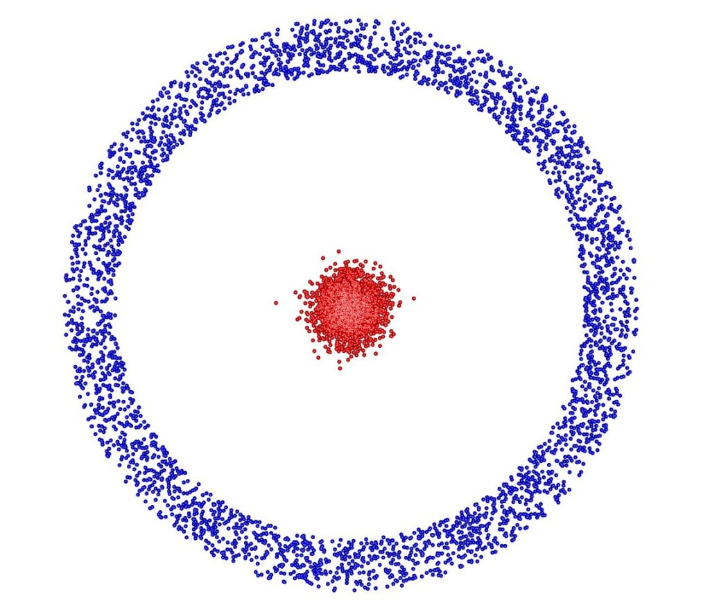 Take the case of the concentric circles, in two dimensions there is clearly no linear function which can make distinct each group. A vanilla k-Means clustering, with the likely segmentation of the data set including all of the inner circle and a slight majority of the outer circle Take the case of the concentric circles, in two dimensions there is clearly no linear function which can make distinct each group. A vanilla k-Means clustering, with the likely segmentation of the data set including all of the inner circle and a slight majority of the outer circle | 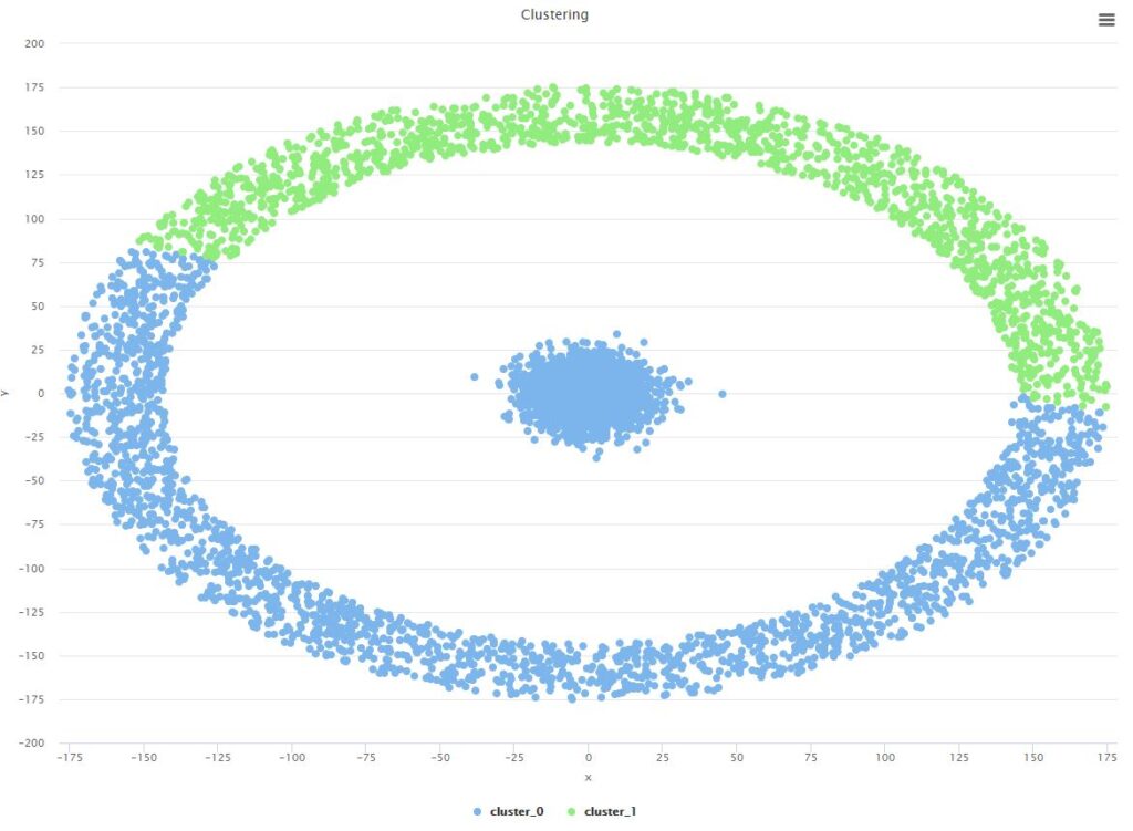 We can see here how the minimisation of the mean squared errors alone is limited in its utility when it comes to identifying the real underlying segments in datasets which are of typologies that are not spherical |
In this instance however it is relatively simple to create a function (ϕ) that allows the clusters to be separated.
e.g.

Using ϕ we can map the 2-dimensional data set that describes the concentric circles on a plane to an appropriate 3-dimensional surface.
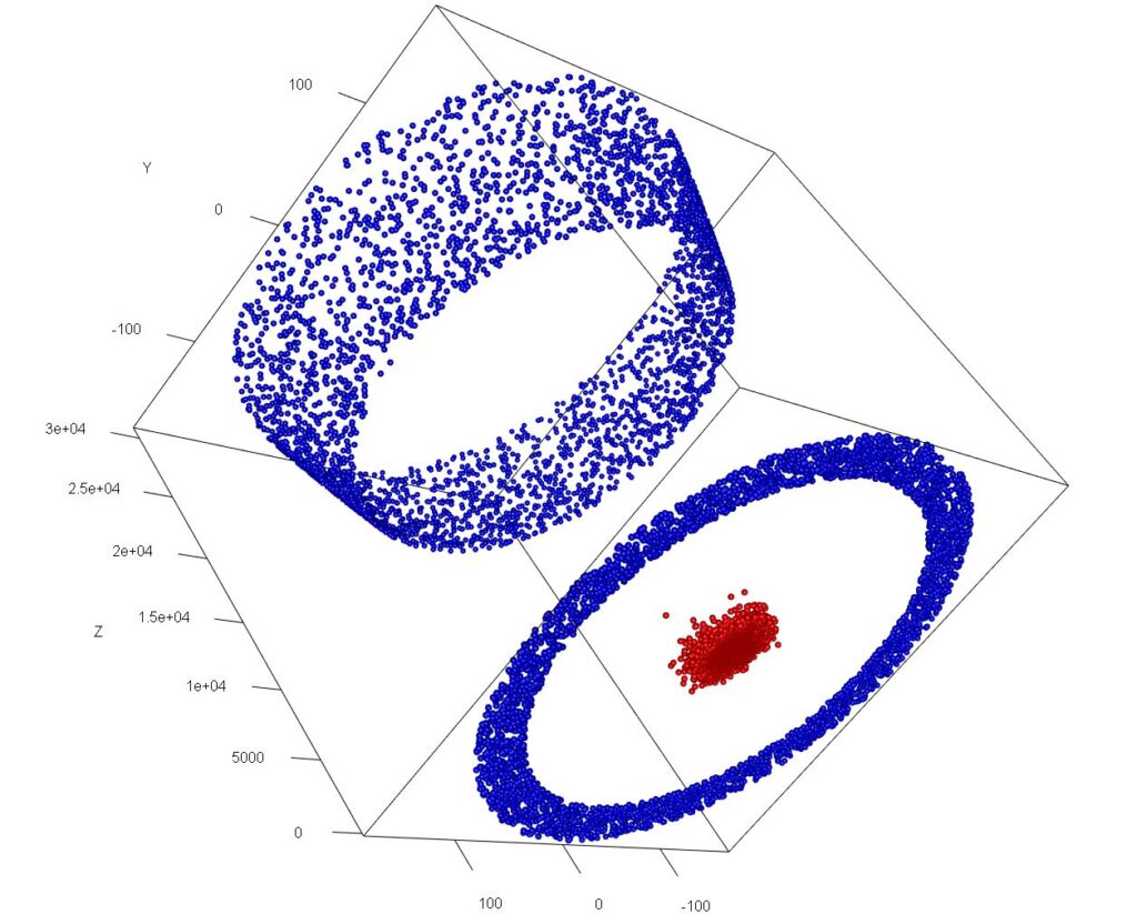 | 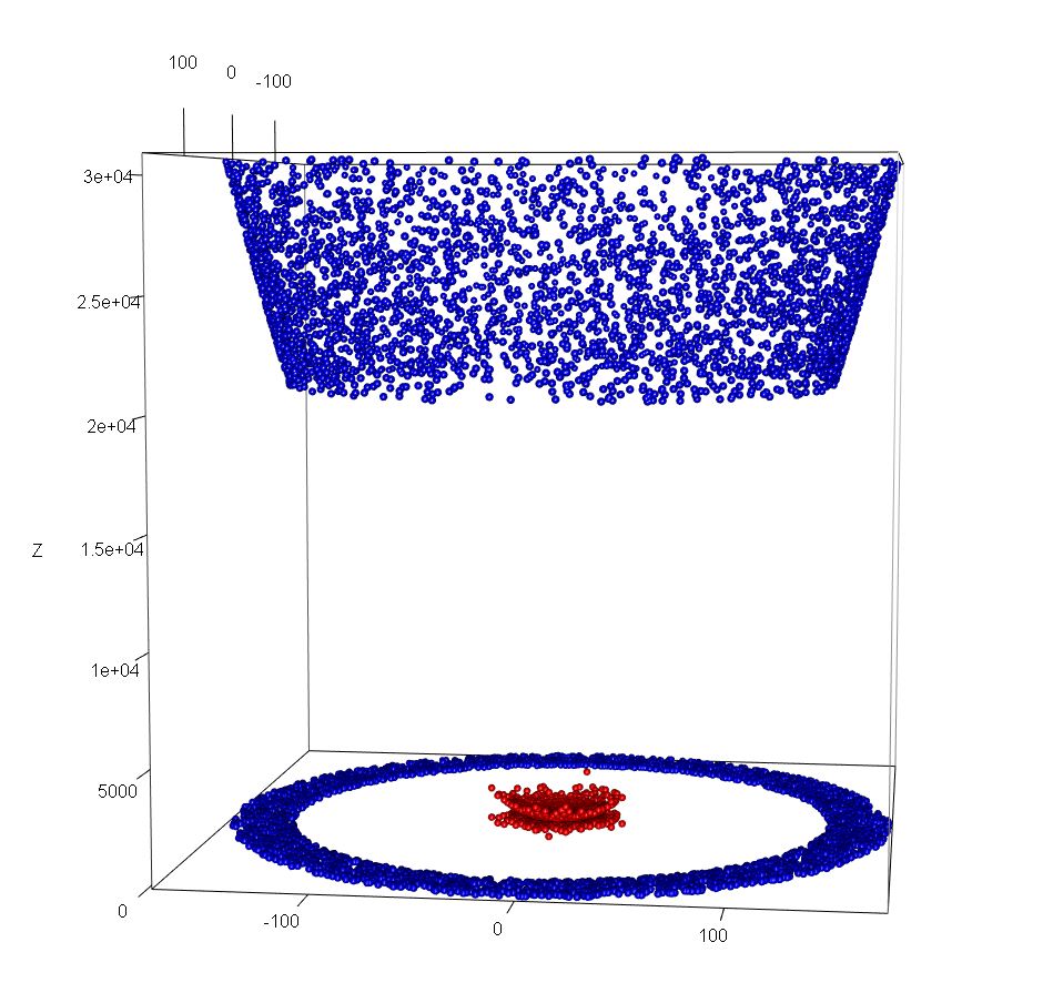 |
As we move into still higher dimensions, while the results are less easily visualised, the principle remains the same. In the above example, for example, any of the two-dimensional planes, parallel to the x,y plane that exists between the highest of the red points and the lowest of the blue points can be used to separate the two clusters (though infinite other boundary descriptions can be described). In higher dimensional spaces we use relatively-lower order surfaces (hyperplanes) to the same effect.

